Factoring in Volatility

Key Points:

• The recent spike in stock market volatility has coincided with a notable correction; such behavior is common in periods of higher turbulence but is typically followed by a bounce back.
• Many factors hold up well in volatile times; others such as small size suffer when volatility spikes but tend to recover as the market calms down.
• Using diversifying factors other than market beta and considering uncorrelated absolute return strategies can benefit a portfolio, both in general and during periods of volatility.

---

Recently, stock market volatility has increased dramatically. Investors are worried about a prospective increase in inflation[i] and analysts have raised the odds of a recession[ii]. Bond yields have gone up[iii] while stocks fell[iv]. Returns of stock indexes have had large swings from day to day and even intraday. The VIX, a measure of expected volatility, surged from 17 at the start of the year to over 50 in early April, a level only seen with the COVID-19 pandemic in 2020 and the Great Financial Crisis of 2008. This spike in volatility has many investors wondering what to expect. In this piece, I examine what high volatility has meant historically for the stock market as a whole and for various market segments.

Historical Volatility

Exhibit 1 shows realized volatility in the U.S. stock market back to July 1963, when data on some of the factors examined later in this piece first become available. I do not use the VIX as it has a shorter history, but results for the common period are qualitatively similar. Volatility here is measured at a monthly level, using the standard deviation of daily returns for the total market. Data through 2024 comes from the Ken French data library[v]; for 2025 I use returns of the Russell 3000 which is a close proxy.

Exhibit 1: Monthly volatility of U.S. stocks, July 1963 – April 2025.

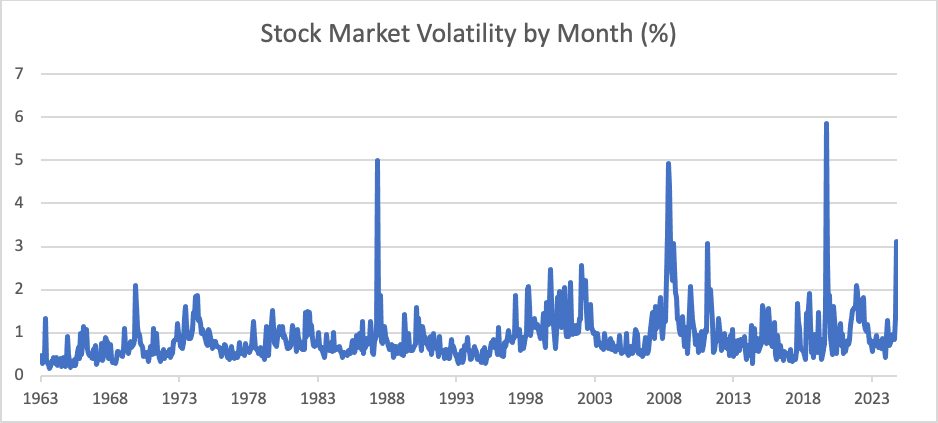
The current spike in market volatility to 3.13% is the fourth highest since 1963. For comparison, the average over this period is 0.87% and the median is 0.72%. The three higher episodes correspond to the Black Monday crash in October 1987, the Great Financial Crisis in 2008, and the onset of the COVID-19 pandemic in early 2020. Some other observational facts stand out. Spikes in volatility can be sudden and sharp but tend to quickly revert to more typical levels. But volatility also tends to be persistent, with elevated levels around those spikes as well as in the Tech Bubble of the late 1990s, while we see other long periods of calmer markets. This pattern is borne out statistically, as the correlation of volatility from one month to the next is 64%. In contrast, the correlation of market returns from one month to the next is only about 3.5%. So if history is any guide, we may expect volatility to come down from its current peak but remain high.

Volatility and Stock Returns

The volatility we are currently experiencing has been accompanied by an overall market downturn. Major indices in the U.S. all suffered corrections and now sit well off their highs. The three other volatility peaks seen in Exhibit 1 all corresponded with bear markets. But we also know that stocks ultimately rebounded, in some cases quite swiftly such as during COVID-19 pandemic times. To gain a better understanding of how general these results are, I examine historical market returns in different volatility regimes.

For this analysis, I categorize all months from July 1963 through December 2024 into one of five buckets, depending on the market volatility that month relative to the full set of months. I will explain how to interpret these exhibits, but readers who do not get enjoyment from tables of numbers can ignore them and simply focus on the explanation in the paragraphs below.

In Exhibit 2 below, the first column of numbers is for the full period, a total of 738 months, or over 60 years. We see the well-known result that stocks have done very well historically, averaging 0.95% monthly returns. These returns have come with some volatility. The monthly standard deviation[vi] is 4.47%, with a minimum of -22.64% and a maximum of 16.61%. Such volatility is why equities command a risk premium, leading to the high and statistically significant (t-stat of 5.76) returns.

Exhibit 2: Monthly returns (in %) of U.S. stocks dependent on volatility, July 1963 – December 2024.

		Same Month Return					Next Month Return
	All	Lo20	Q2	Q3	Q4	Hi20	Lo20	Q2	Q3	Q4	Hi20
Mean	0.95	1.92	1.73	1.48	0.66	-1.05	0.82	0.87	0.68	1.16	1.23
Stdev	4.47	2.56	3.12	3.75	4.37	6.69	2.98	3.32	4.37	4.92	6.08
Count	738	148	147	148	147	148	148	147	148	146	148
T-stat	5.76	9.13	6.71	4.79	1.83	-1.90	3.34	3.17	1.88	2.84	2.46
Min	-22.64	-4.10	-6.67	-10.50	-11.23	-22.64	-7.49	-8.15	-12.19	-22.64	-17.15
Max	16.61	8.58	9.10	12.63	12.89	16.61	8.58	11.90	12.89	11.89	16.61

Source: Ken French data library, Bridgeway calculations

The next set of five columns gives monthly stock returns depending on volatility that month. The lowest quintile or 20% of months by volatility are on the left, the most volatile quintile is on the right, and the intermediate quintiles are in between. Average returns monotonically decrease as volatility increases: Stocks return 1.92% in the 148 months when volatility is lowest, declining to a loss of 1.05% in the 148 months when volatility is highest. The market declines we saw with the biggest spikes in volatility hold more generally when volatility is elevated. Not only is the average monthly return of -1.05% significant with a t-stat of -1.90, it is even more significant relative to the overall average market return of 0.95%.

While these results hold on average, they are by no means a guarantee, with plenty of variation in all volatility environments. Unsurprisingly, that variation is greatest when volatility is highest, with a standard deviation of 6.69% and the most extreme minimum and maximum returns. But even the calmest months provide a wide range of outcomes. Returns can be nicely positive or disappointingly negative in all volatility environments.

These results help explain current returns based on volatility, but what about future market returns? This question is addressed in the final five columns. Here I look at the volatility in a given month and show the next month’s returns. The picture is different. Most notably, the highest returns occur following months with the highest volatility, exactly opposite same month returns. Variations do persist, as seen by the continued higher standard deviations and return spreads in the month after high volatility. But as volatility subsides, the market tends to recover, sometimes quite strongly as seen for example after the big volatility spikes from the Great Financial Crisis and COVID-19 pandemic. Indeed, at the end of April 2025, markets partly recovered from the earlier lows of the month. This pattern is a cautionary tale for those tempted to sell when markets fall and get volatile.

Volatility and Segments of the Market

These results show how the stock market as a whole performs across volatility regimes, but what about different segments of the market? Perhaps some do better than others in periods of high volatility?

I first examine the performance of factors — groups of stocks defined by certain characteristics. For example, a common academic version of the value factor, HML, is given by the return of the highest 30% of stocks by book-to-market (B/M) minus the lowest 30%. Making use of factors in forming portfolios not only gives the potential for higher returns, but also provides a more diversified portfolio[vii]. I use common definitions from the Ken French data library, but variations are possible. For example, making use of multiple metrics (e.g. including earnings, sales and cash flow relative to price in value) or using contextual definitions can improve factor performance. I show only the average returns by volatility environment to save space, but suffice it to say that again there is plenty of variation around those averages[viii], which makes trying to time these factors difficult.

Exhibit 3: Monthly factor returns (in %) of U.S. stocks dependent on volatility, July 1963 – December 2024. Factor definitions are given in the text.

		Same Month Return					Next Month Return
	All	Lo20	Q2	Q3	Q4	Hi20	Lo20	Q2	Q3	Q4	Hi20
Mkt – Rf	0.58	1.59	1.31	1.07	0.29	-1.34	0.48	0.46	0.27	0.77	0.94
SMB	0.17	0.78	0.12	0.26	0.18	-0.52	0.18	-0.02	0.22	-0.01	0.46
HML	0.28	0.33	0.12	0.27	0.37	0.30	0.38	0.39	0.41	0.12	0.09
RMW	0.28	0.09	0.31	0.12	0.43	0.48	0.19	0.23	0.24	0.67	0.10
CMA	0.26	0.05	-0.06	0.12	0.38	0.79	0.14	0.13	0.30	0.22	0.49
UMD	0.61	0.89	0.64	1.01	0.55	-0.02	0.82	0.86	0.91	0.81	-0.34
STREV	0.44	0.56	0.54	0.37	0.35	0.39	0.25	0.23	0.10	0.48	1.14
DYLD	0.03	-0.35	-0.19	-0.34	0.28	0.75	0.04	0.08	0.11	-0.13	0.05

Source: Ken French data library, Bridgeway calculations

The top row of numbers is the market beta factor or equity risk premium, which measures the return of the stock market relative to the risk-free rate of cash, as represented by one-month Treasury bills. We see a very similar picture as in Exhibit 2: stocks do best relative to cash in low volatility months and worst in high volatility months. But in the month after high volatility, stocks outperform the most.

The next two factors, SMB and HML, represent the excess returns of small size and value. These factors form the core of many academic factor pricing models and are the basis for common equity portfolio classifications such as small value or large growth funds. When volatility is high, riskier small stocks tend to suffer and lag larger stocks. But these beaten-down small stocks typically recover much of those losses in the following month. Value stocks, on the other hand, display no notable pattern, generally doing well no matter the volatility environment. In the month following high volatility episodes, value excess returns tend to be weaker but are still positive.

RMW represents the premium of stocks with robust versus weak profitability. While always positive no matter the volatility environment, it performs best when volatility is high and investors might seek higher quality companies with better profitability. As seen with other measures, this behavior reverts in the following month to a lower albeit positive premium. CMA refers to the premium of stocks with more conservative growth in assets relative to firms that are more aggressive. Again we see a flight to quality in times of higher volatility, which while lower the following month, remains higher than other volatility environments as well as the overall average.

The following two factors are based on return patterns. UMD measures medium-term momentum and STREV gives one-month reversals. Momentum is strong overall except in months of high volatility and the subsequent month as well. This is consistent with the findings and explanation of “When and Why Does Momentum Work – and Not Work?”[ix] which noted that volatile markets can disrupt the trend following that momentum relies upon. Conversely, short-term reversals perform best in the month after high volatility. This is consistent with what we saw for the stock market overall. On average, the market falls when volatility spikes but then reverses the next month. Similarly, those individual stocks which performed worst subsequently rebound the most in the following month.

I also examined sector returns; results are not shown for brevity. For every sector, returns were by far the worst when volatility was highest, and for all but one sector those returns were negative. This one exception was Utilities, which also had its worst returns when volatility was high, but they were still positive. Utilities tend to pay high dividends, and their returns align with what we see for dividend yield in the final row of Exhibit 3. In times of turmoil, investors tend to seek out the relative safety of higher dividends.

Implications for Investors

The recent spike in market volatility is the fourth highest in the past 60 years and has coincided with a stock market drawdown. Such behavior is typical for periods of higher volatility. Higher volatility and drawdowns are features of the stock market, and lead to the equity risk premium – the long-term outperformance of stocks over less risky investments. Indeed, in the subsequent month after high volatility, stocks as a whole tend to recover, as do beaten down segments of the market such as smaller stocks.

One important implication for investors is to be wary of making big moves when volatility has soared and stocks have dropped. You could well be locking in those losses and risk missing out on the subsequent recovery. A disciplined, systematic approach can help avoid the temptation to make kneejerk reactions. Investors should build a well-diversified portfolio that can help them withstand, both financially and emotionally, the inevitable shocks that arise. Diversification can be from other asset classes; it can also come from utilizing other factors besides market beta as sources of return. Most of these factors hold up well on average both overall and during periods of high volatility. Disciplined rebalancing and appropriate risk controls can help preserve the power of diversification and reduce downside risk during volatile times. Investors may also want to consider an allocation to absolute return strategies that are uncorrelated to the market. Keeping these points in mind can help you stay calm during periods of turbulence.

---

[i] See https://bridgeway.com/perspectives/factoring-in-inflation/ for a discussion of inflation and investing.

[ii] See https://bridgeway.com/perspectives/stress-test-how-factors-perform-before-during-and-after-recessions/ for a discussion of investing around recessions.

[iii] See Berkin, Andrew L. 2018. “What Happens to Stocks When Interest Rates Rise?” Journal of Investing 27 (2): 126-135.

[iv] See https://bridgeway.com/perspectives/factoring-in-bear-markets/ for a discussion of investing in a bear market.

[v] https://mba.tuck.dartmouth.edu/pages/faculty/ken.french/data_library.html.

[vi] Note this is the standard deviation of monthly returns over the full set of 738 months. This is different from the calculation of market volatility of Exhibit 1, which gives the standard deviation of daily returns for each month.

[vii] See “Your Complete Guide to Factor-Based Investing: The Way Smart Money Invests Today” by Andrew L. Berkin and Larry E. Swedroe, BAM Alliance Press, 2016 for a discussion of factors and their use in forming a more diversified portfolio.

[viii] The full set of results is available upon request.

[ix] Berkin, Andrew L. 2021. “When and Why Does Momentum Work – and Not Work?” Journal of Investing 30 (5): 35-54.