Recently the large cap US S&P 500 index hit an all-time high, closing above its previous high set two years ago in January 2022. Does this mean the S&P 500 is due for an imminent crash?
In the 1920s radio was the hot technology and the stock prices of associated companies soared. The poster child was the Radio Company of America (RCA), whose price rose from $43 a share in 1926 to a peak of $568 in September 19291, with a P/E ratio of 722. The stock market crash that commenced with Black Monday that month brought RCA’s stock price back to Earth, falling to $15 in 1932. It wasn’t until the 1960s that RCA regained its former high. A presumably apocryphal story is of an older man going to a brokerage to sell his long-held RCA shares, proclaiming, “Even money!” Needless to say, having an investment return of nothing for over three decades is not desirable.
Fast forward to the 1980s. Japanese technology, manufacturing, and real estate are on top of the world. On December 29, 1989, Japan’s benchmark Nikkei 225 hit an all-time high of 38,915.87, with a forward P/E ratio of over 503. Japan’s bubble economy subsequently burst, and the Nikkei fell sharply, dropping below 7,000. Fast forward again to recent times. On February 22, 2024, the Nikkei 225 closed at 39,098.68, finally breaking through its prior record high. After a span of over three decades, “Even money!”
Recently the large cap US S&P 500 index also hit an all-time high, closing above its previous high set two years ago in January 2022. Does this mean the S&P 500 is due for an imminent crash? The answer is no. The S&P 500 may fall or rise from here, but hitting an all-time high will not be the reason4. Since stocks tend to go up over time, all-time highs are common events. RCA and the US market hit many all-time highs before crashing in 1929; similarly with the Nikkei prior to its crash in 1989. In those cases, the rise in prices eventually far outstripped the rise in fundamentals, such as earnings, leading to extreme valuations. While the valuation of the S&P 500 today is elevated relative to history, it is below levels of a few years ago as well as in 1929 and 20005.
An important takeaway is that valuations do matter. Certainly, other factors such as quality and sentiment also drive returns, which is why we use them as well as value. Stocks can be cheap for a reason; they can also be expensive for a reason. And there were good reasons for the initial rise of both RCA and the Nikkei. RCA was a leader in both radio manufacturing and broadcasting, hot growth areas at the time. The Japanese economy boomed in the 1980s as exports soared. But as the Wall Street saying goes, “trees don’t grow to the sky”. At some point, stocks can get too expensive, and subsequently fall precipitously6.
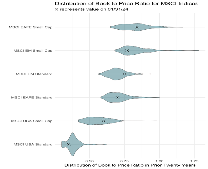
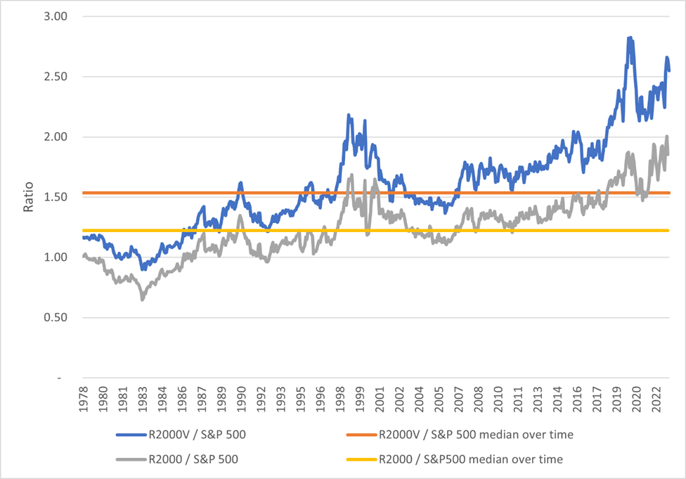
If valuations matter, where can one find attractive valuations today? One place is smaller cap stocks, whose returns have lagged their larger cap peers in recent years. Around the world, smaller cap stocks are priced more attractively relative to fundamental measures of value than their larger brethren. This holds true in the United States, other developed markets, and emerging markets. For example, the figure below shows that using Book to Price as a value measure, US small caps are cheaper than US large caps, EAFE (developed markets) small caps are cheaper than EAFE large caps, and EM small caps are cheaper than EM large caps. As noted, valuation is not the only driver, and there are other reasons why smaller cap stocks are attractive. We have discussed the case for smaller cap stocks in the United States7 and emerging markets8 in some recent pieces.
Source: FactSet, Bridgeway analysis
Value stocks do tend to have higher subsequent returns than their more expensive peers, a finding that goes back to at least Benjamin Graham9. For stock indices, Robert Shiller showed cheaper valuations tend to produce higher return over the next ten years (see footnote 5). Thus, valuations can be useful for setting long-run return expectations but have less short-term effect. Structural issues such as liquidity and legal protections also affect valuation levels. For example, the United States tends to have higher valuations than other markets. But if you believe in value investing, small caps are an interesting opportunity.
Note this is not a call to make a major tactical asset allocation shift. As always, diversification is important. And timing shifts in the market is nigh impossible. But for those whose allocation to small caps has moved away from target due to the run up in large cap stocks, rebalancing is well warranted. Given the discrepancy in valuations, investors may wish to revisit their return assumptions and consider an increased allocation to smaller stocks. And for those who have been ignoring smaller cap stocks in any of these markets, now is a good time to consider adding this asset class to your allocation.
See for example “Bubbles and Crashes: The Boom and Bust of Technological Innovation” by Brent Goldfarb and David A. Kirsch. Prices are split adjusted. ↩︎
For a thorough discussion of value, as well as other factors, see “Your Complete Guide to Factor-Based Investing: The Way Smart Money Invests Today” by Andrew L. Berkin and Larry E. Swedroe. ↩︎
DISCLAIMER AND DISCLOSURE
The opinions expressed here are exclusively those of Bridgeway Capital Management (“Bridgeway”). Information provided herein is educational in nature and for informational purposes only and should not be considered investment, legal, or tax advice.
Past performance is not indicative of future results.
Investing involves risk, including possible loss of principal. In addition, market turbulence and reduced liquidity in the markets may negatively affect many issuers, which could adversely affect client accounts.
Diversification neither assures a profit nor guarantees against loss in a declining market.
The Price-to-Earnings (P/E) Ratio is the ratio for valuing a company that measures its current share price relative to its earnings per share (EPS). The price-to-earnings ratio is also sometimes known as the price multiple or the earnings multiple.
The book-to-price ratio is a financial metric that compares a company’s current book value to its market value. It’s calculated by dividing the book value per share by the current stock price per share.
The Nikkei 225, also commonly referred to simply as the Nikkei or the Nikkei index, is the leading stock market index for Japan. It tracks the performance of 225 large, publicly traded companies listed on the Tokyo Stock Exchange (TSE).
The S&P 500 Index is a broad-based, unmanaged measurement of changes in stock market conditions based on the average of 500 widely held common stocks.
The MSCI EAFE Standard, also known as the MSCI EAFE Index, is an equity index that captures large- and mid-cap representation across 21 developed markets countries around the world, excluding the US and Canada. The MSCI EAFE Small Cap Index is an equity index that captures small cap representation across developed markets countries around the world, excluding the US and Canada.
The MSCI USA Standard, also known as the MSCI USA Index, is designed to measure the performance of the large- and mid-cap segments of the US market. The MSCI USA Small Cap Index is designed to measure the performance of the small-cap segment of the US equity market.
The MSCI EM Standard, also known as the MSCI Emerging Markets Index, captures large- and mid-cap representation across 24 emerging markets countries. The MSCI Emerging Markets (EM) Small Cap Value Index captures small-cap securities exhibiting overall value style characteristics across 24 emerging markets countries.
One cannot invest directly in an index. Index returns do not reflect fees, expenses, or trading costs associated with an actively managed portfolio.
In their 2020 book The Incredible Shrinking Alpha[1], Larry Swedroe and Andrew Berkin noted, “The financial equivalent of the quest for the Holy Grail is the quest for money managers who will deliver alpha, defined as returns above the appropriate risk-adjusted benchmark.” Alpha is typically measured as returns unexplained by conventional academic models using factors such as the market, size, value, momentum, profitability, and quality for equity portfolios[2]. The book provides the reasons and evidence for why alpha has been shrinking.
Many money managers work tirelessly seeking this elusive alpha. Yet, in this piece, we claim that there is, in fact, alpha to be found in a more straightforward manner. Does this contradict the Incredible Shrinking Alpha book? The answer is no. Rather than toiling over idiosyncratic name-by-name stock selection or trying to time the market, this incredible structural alpha can be found with thoughtful consideration of the factors driving returns and the portfolios designed from them.
This piece is a shorter version of a full paper with more details. We include two exhibits. Panel A of Exhibit 1 shows annualized returns of a 5×5 grid of all US stocks listed on major stock exchanges with positive book value, sorted on size and value as measured by book to market (B/M). High (low) B/M refers to the deepest (least) value stocks by this measure. A few features stand out. The smallest and deepest value stocks in the lower right have the highest returns at over 16% annually. In contrast, the smallest low value stocks in the lower left corner have the lowest returns. Generally, the deepest-value stocks in the right column have higher returns than the low-value stocks in the left column. The exception is for the largest quintile of stocks in the top row, where the returns are comparable. Value as measured by B/M has paid off over the long term, except for the largest stocks. Generally, smaller size has paid off too, and the smallest deepest value stocks have the highest returns.
Exhibit 1:
Source: S&P Compustat, CRSP, and Bridgeway calculations
We’ve been looking at returns, but what about alpha or risk-adjusted returns? To measure alpha, we adjust using a Fama-French-Carhart four-factor model to see what returns are unexplained by the market, size, value, and momentum. Results are in Panel B. For the largest stocks, the low value stocks have positive alpha while high value has negative alpha, despite their comparable returns. The largest low (high) value stocks have exceeded (lagged) return expectations based on their B/M characteristics. Meanwhile, we find that the smallest and deepest value stocks indeed have strong and statistically significant alpha. These stocks have excess returns beyond what one might expect from their small and deep value characteristics; portfolios constructed with greater weight to this segment of the market would benefit from these higher-than-expected returns.
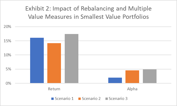
Delving deeper into the smallest and deepest value portfolio, Scenario 1 of Exhibit 2 (blue bars) represents the typical academic protocol used for factor models of rebalancing just once a year. But new data comes in constantly. Scenario 2 (the orange bars) shows what happens when we rebalance quarterly and use timely price information. Compared to Scenario 1, more timely data increases alpha by over 2.5% annually. These are extra returns not captured by the slower-moving academic factor models.
Exhibit 2:
Source: S&P Compustat, CRSP, and Bridgeway calculations
But note that the raw returns decrease by almost 2%. Why? The reason is momentum. By rebalancing more frequently, we include more stocks that have recently dropped in price and thus have negative momentum. Now, alpha is nice, but at the end of the day, what investors can spend is the raw return. A way out of this problem is to screen the portfolio for these “falling knives” and avoid buying stocks that have seen large price drops. This helps remove the unwanted exposure to negative momentum.
Book to market is just one way to measure value, but there are others. Scenario 3 (grey bars) forms a “combo” value measure using B/M, sales to price, earnings to price, and cash flow to price as well as screens out the worst quintile of momentum names. This combo measure uses data from the balance sheet, top and bottom of the income statement, and the statement of cash flows. While returns from these measures are correlated, combining them provides diversification benefits. Returns and alpha both increase notably. Why does this extra return also manifest itself as alpha? It’s because the factor model is based just on B/M; this structural switching to multiple value metrics provides a boost not captured by B/M alone.
This momentum screen is one example of avoiding groups of stocks to provide structural alpha. In a similar manner, one can also avoid stocks with poor profitability. One can also avoid other “bad actors” such as penny stocks, recent IPOs, stocks with high costs to borrow, and stocks in bankruptcy.
Implementation matters tremendously as well. Poor implementation can hurt returns and alpha; disciplined implementation can be additive to both. This means trading patiently, providing liquidity to the market. Having a good number of stocks to choose from helps greatly, rather than needing to trade in a set of given names. Setting bounds on individual positions and sector weights aids in keeping a diversified portfolio while still targeting the desired factors. And securities lending brings in extra returns, especially in market segments like small value where a greater number of hard-to-borrow stocks are located.
Finally, one may wonder, if this is structural alpha, can one structure an index fund to access it? For existing index funds, the answer is an emphatic no! Most indexes don’t target the smallest deepest value stocks we highlight here, and many index providers use only B/M as their value measure and reconstitute their indexes less frequently. Furthermore, all index funds must buy the exact stocks at the exact weights on the exact dates, which doesn’t necessarily allow for the most efficient implementation. But managers actively targeting their desired exposures and actively managing their implementation can certainly attain this structural alpha.
While alpha from market timing and individual stock selection may be shrinking, one can still add value by targeting the factors that provide a premium. And as we have shown in this article, one can further add alpha above the returns explained by these factors. The sources of this alpha include deeper factor exposure, multiple metrics to evaluate a factor, timely rebalancing of portfolios, taking other factors such as momentum into consideration, avoiding bad actors, and disciplined implementation. These are some of the many details Bridgeway considers when constructing thoughtfully structured portfolios. We believe these details are worthwhile and we continue to pursue the research and discipline required to achieve this structural alpha.
The opinions expressed here are exclusively those of Bridgeway Capital Management (“Bridgeway”). Information provided herein is educational in nature and for informational purposes only and should not be considered investment, legal, or tax advice.
Past performance is not indicative of future results.
Investing involves risk, including possible loss of principal. In addition, market turbulence and reduced liquidity in the markets may negatively affect many issuers, which could adversely affect client accounts.
Diversification neither assures a profit nor guarantees against loss in a declining market.
The book to market ratio compares a company’s book value to its market value. The book value is the value of assets minus the value of the liabilities. The market value of a company is the market price of one of its shares multiplied by the number of shares outstanding.
The sales to price ratio is a valuation ratio that compares a company’s revenue to its stock price It is an indicator of the value that financial markets have placed on each dollar of a company’s sales or revenues.
The earnings to price ratio is the ratio for valuing a company that measures its earnings per share (EPS) relative to its current share price. The earnings-to-price ratio is also sometimes known as the price multiple or the earnings multiple.
The cash flow to price ratio is a stock valuation indicator or multiple that measures a company’s operating cash flow per share relative to its stock price. The ratio uses operating cash flow (OCF), which adds back non-cash expenses such as depreciation and amortization to net income.
Following up on our analysis of factor performance in rising interest rates1, recessions2, and bear markets3, we discuss the benefits of remaining invested in stocks and maintaining multi-factor diversification to help weather periods of high inflation.
After years of laying low, inflation emerged in 2021 and has remained elevated. In the United States, the annual rate of inflation as measured by the Consumer Price Index (CPI) was 3.7% as of September 2023. That’s down from its peak of 9.1% in June of last year, but still well above the rates we typically saw during the previous 10 years, when inflation rarely edged much higher than 2%.
We haven’t seen inflation numbers like these since the early 1980s, before the experience of many of today’s investors. The Federal Reserve has been raising interest rates in response. Both the S&P 500 and U.S. Treasuries fell in 2022 as yields rose; while the stock market has recovered this year, bond prices have continued their fall.
The situation is similar around the world, with inflation spiking and markets having fallen. There are a multitude of potential reasons for inflation’s unwelcome return, including ongoing supply chain issues that have made goods scarce, stimulus money that gave consumers more dollars to go after fewer goods, pent-up spending demand unleashed after the pandemic, a decades-long low-interest rate environment and deficit spending. But investors may be less concerned about the causes of inflation than they are about its impact on their portfolios.
Does high inflation always cause markets to drop? We don’t have to look very far back for a counterexample. Inflation was 7.0% in 2021 yet the S&P 500 soared by 28.71%. Contrary to screaming headlines, stocks can do quite well — as well as poorly — during high inflationary periods. That raises important questions about the actual relationship between inflation and stock performance.
In this piece, we examine how stocks have performed historically in different inflationary environments and compare them to the asset classes of bonds and cash. We start by giving brief conceptual arguments before examining historical data going back over a century. We next look at how different segments of the market, such as factors and sectors, have performed. To get even more data and show the robustness of our results, we then extend our work to over 20 developed markets. Finally, we close with some takeaways to guide investors looking ahead.
The highlights: Higher inflation isn’t always bad news for stocks, and it can affect the performance of different factors quite differently. And even when high inflation dampens equity returns, stocks still produce positive returns on average during high inflationary periods—and strongly outperform cash.
These results suggest that investors who let fears of high inflation drive them out of the stock market could be making a costly mistake.
How Might We Expect Markets to React to Inflation?
Reasons why inflation is bad for the stock market often involve that the central banks, such as the U.S. Federal Reserve, will raise interest rates to slow the economy and fight inflation. This slowing of the economy then leads to lower stock prices. Rising interest rates also bring higher discount rates, leading to lower stock valuations. But as we showed (see footnote 1), while higher rates do bring lower bond returns due to the bond math, there is no distinct relation with stock returns. Interest rates will rise because of a strong economy, which should bring higher earnings and cash flows.
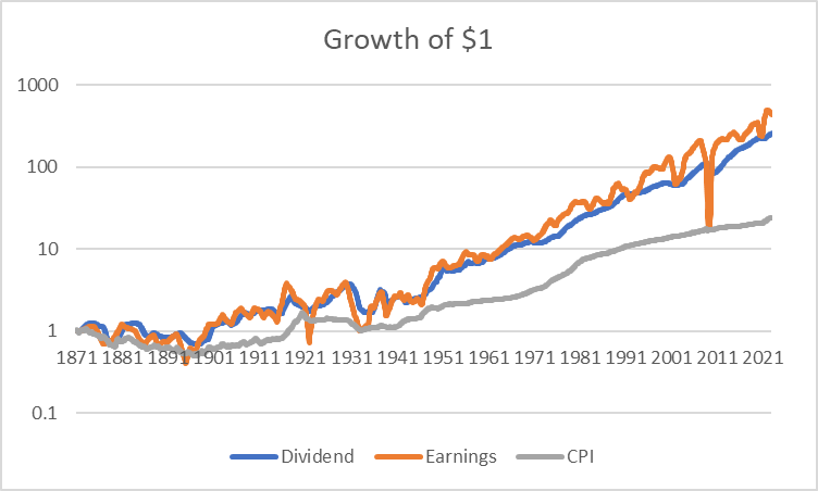
This argument is behind why some argue that stocks should provide a good inflation hedge. As prices in general go up, so should the sales, earnings, cash flows, and dividends of the companies in the stock market. Provided valuations such as P/E ratios stay the same, stocks should be a good match for inflation. We can see this in Exhibit 1, which uses over 150 years of US data from Robert Shiller’s website4. The plot shows the growth in earnings, dividends, and inflation from 1871 through 2022. Visually we get a long-term perspective. Earnings and dividend growth indeed track inflation over time, but at a higher level. This makes sense. Stocks allow the investor to participate in the growth of the economy, and that nominal growth has typically been higher than inflation. Recall that the most common measure of economic growth, gross domestic product or GDP, is typically given in real terms, meaning after inflation.
Exhibit 1: Growth of $1 in CPI, Dividends, and Earnings, 1871 – 2022
Source: Robert Shiller, Bridgeway calculations
Exhibit 2 puts numbers to the visual and moves to a yearly time frame by giving the correlation of inflation, earnings, dividends, and stock returns for the US. Inflation correlates at 27% and 20% with annual changes in dividends and earnings, respectively. This is modestly positive, but recall that earnings are smoothed by accounting items such as depreciation, amortization, and accounts receivable and payable. Dividends are discretionary, and companies smooth them in order to avoid dividend cuts, which are viewed poorly by the market. Such smoothing can reduce the correlation of earnings and dividends with inflation. Stock returns are even more modestly correlated with inflation at 13%. This is still positive, so stocks do provide a modest hedge to inflation at an annual level. But there is more going on, as the market is forward-looking and moves to perceptions of future cash flows and discount rates. With that said, let’s next look at how asset classes respond to inflation.
Exhibit 2: Correlations of Annual Changes in CPI, Dividends, Earnings and Stock Returns, 1871 – 2022
CPI
Dividends
Earnings
Returns
CPI
1
0.27
0.20
0.13
Dividends
0.27
1
0.19
0.06
Earnings
0.20
0.19
1
0.29
Returns
0.13
0.06
0.29
1
Source: Robert Shiller, Bridgeway calculations
Stocks and Inflation in the U.S.
We start by examining how the United States stock market fares compared to the risk-free rate in different inflationary regimes. Inflation data is released monthly with a lag and is often subsequently revised. We avoid shorter-term timing and focus on annual returns. Such longer time frames lessen the impact of noise from short-term fluctuations, the details of timing, and transaction costs. Return data comes from the Ken French data library5, while inflation comes from the Federal Reserve6. We go from the start of annual returns in 1927 through 2022, giving us a 96-year history.
Exhibit 3 shows the returns of US stocks and the risk-free rate (cash, as given by one-month T-bills) according to the same year’s level of inflation. While we explain how to interpret these exhibits, readers whose eyes glaze over at tables of numbers can ignore them and simply focus on the explanation in the paragraphs below.
There are three sets of five columns. The three sets give the amount of inflation, stock market returns, and risk-free returns. The five columns represent different quintiles of inflation; the 19 years of lowest inflation are on the left, while the 20 years of highest inflation are on the right. By definition, average inflation increases from -1.52% in the lowest inflation quintile to 8.63% in the highest quintile. From the “Min” row, inflation of 4.86% or higher puts a year in the highest quintile. The 7.04% and 6.45% inflation of 2021 and 2022 are solidly into the highest quintile of inflation, for example, although well below the all-time high of 18.13% (reached in 1946 as prices spiked in the aftermath of World War II). The next five columns show stock returns grouped according to inflation quintiles, while the last five columns show cash as given by the risk-free rate, also grouped according to inflation quintiles.
Exhibit 3: Stock and Risk-free Returns Dependent on Same Year Inflation (all in %) 1927-2022
Source: Ken French data library, Federal Reserve FRED data library, Bridgeway calculations
We can see that stock returns are consistently positive in each of the five inflationary regimes. However, there is great fluctuation, as seen by the high standard deviations and the spread of the minimum and maximum returns. Returns are highest and quite statistically significant for the middle three inflationary quintiles. Stocks are not as strong on average when inflation is low or negative. This aligns with our argument that stocks might follow prices; when sales and earnings are kept low by deflation, there is little growth to reflect in stocks.
When inflation is highest, stock returns are still nicely positive at 5.84% annually. High inflation does not necessarily mean that stocks will fall; indeed, on average they do just fine. But our caveat of great fluctuations still applies here; in any given year results could be much better or much worse.
Also, note that the average return is not just nicely positive, it is also higher than the average short-term interest rate of 5.03%. Investors who panic about their stock holdings and move into cash when inflation is high tend to do worse. In fact, the term “risk-free” rate is a misnomer from a real inflation-adjusted perspective. When inflation is high, holding cash doesn’t keep up with rising prices, and investors lose purchasing power. On average, stocks also lag inflation when the latter is high, but they do outperform cash.
One could wonder, if I see high inflation now, what will happen in the future? We address this in Exhibit 4. The first five columns tell us the level of inflation based on the inflation of the prior year. We still see that the averages move from low to high as we go from quintile 1 to quintile 5. Inflation is sticky; high or low inflation in one year tends to be repeated the next year. But it is not guaranteed. For example, the highest annual inflation of 18.13% in 1946 is now in the middle quintile, as it followed the moderate 2.25% inflation of 1945.
What is of particular interest to the investor is what happens to stocks and cash. After a year of high inflation, stocks now do quite well, with an average return of 11.07%. This is on par with the returns of the other quintiles, as well as the long-term average of 11.84% for this period. There is plenty of variation from year to year, as can be seen from the standard deviation as well as minimum and maximum, but this is always true for stocks. Cash yields remain elevated in years following high inflation, as the Fed keeps rates elevated. But now, those cash returns are trounced on average by the return of stocks. The upshot for investors? If you pull out of stocks because inflation is high, not only do you get worse returns on average in the current year, but you also risk missing out on the subsequent strong performance of stocks in the following year.
Exhibit 4: Stock and Risk-free Returns Dependent on Prior Year Inflation (all in %) 1927-2022
Source: Ken French data library, Federal Reserve FRED data library, Bridgeway calculations
Inflation and Segments of the Market
While those results make a case that the stock market as a whole delivers positive returns across inflationary regions, what about different segments of the market? Perhaps some do better than others in periods of high inflation?
We first examine the performance of factors — groups of stocks defined by certain characteristics. For example, a common academic version of the value factor, HML, is given by the return of the highest 30% of stocks by book-to-market (B/M) minus the lowest 30%. We use common definitions from the Ken French data library. We show only the average returns by inflationary regime to save space, but suffice it to say that again there is plenty of variation around those averages.
Exhibit 5: Average Factor Returns (%) Dependent on Same Year Inflation (1927-2022 for Mkt-Rf, SMB, HML, and UMD) (1964-2022 for RMW and CMA)
Infl Lo20
Infl Q2
Infl Q3
Infl Q4
Infl Hi20
Mkt – Rf
7.47
14.29
12.20
8.39
0.81
SMB
0.83
5.23
4.84
3.20
0.60
HML
0.23
2.68
4.16
5.58
9.26
UMD
11.65
8.35
4.98
10.87
9.49
RMW
5.69
-0.34
2.91
6.31
3.39
CMA
-2.00
4.52
2.72
2.59
6.75
Source: Ken French data library, Federal Reserve FRED data library, Bridgeway calculations
The first row (Mkt-Rf) is simply the equity risk premium — the market’s return relative to the risk-free rate. It is the same as subtracting the appropriate two columns in Exhibit 37, and highlights that excess stock returns are lowest when inflation is high, but still positive.
The remaining rows show how different factors perform in different inflationary environments (again grouped by quintile). For example, smaller stocks always show a premium, but it is lower when inflation is either very high or low. Most other factors8 demonstrate no clear pattern, with one notable exception: Value.
As inflation increases, the value premium (as represented by HML) increases as well in a monotonic fashion. This is in exact agreement with what we showed by looking at decades from our perspective Does Value Just Need Some Growth?9 While there is plenty of variation (not shown to save space), on average, value performs best when inflation is higher.
We look at returns by sector in Exhibit 6. Generally, returns are lowest in the low and high inflation quintiles, in keeping with the overall pattern of the market returns we saw in Exhibit 3. Otherwise, there is again little noticeable pattern, with the exception of Energy. For this sector, returns rise monotonically with inflation, climbing from 4.89% on average in the low inflation quintile to 21.42% when inflation is high. This perhaps reflects the special role of energy in powering the economy and helping to drive consumer prices. Certainly, the Energy Crisis of the 1970s drives some of this behavior, but we see a similar pattern in other periods of high inflation, as well as currently.
Exhibit 6: Average Sector Returns (%) Dependent on Same Year Inflation (1927-2022)
Infl Lo20
Infl Q2
Infl Q3
Infl Q4
Infl Hi20
Nondurables
9.04
15.67
11.81
20.26
5.06
Durables
20.04
30.02
15.20
10.10
4.46
Manufacturing
10.52
16.90
17.27
15.23
5.78
Energy
4.89
8.99
11.63
18.10
21.42
Chemicals
15.61
14.45
12.13
14.97
5.93
Business Equipment
11.96
20.17
23.60
12.31
4.60
Telecom
6.83
17.29
16.44
10.40
2.50
Utilities
7.91
10.58
15.82
15.94
5.62
Shops
11.46
22.09
11.18
18.81
3.33
Health
10.08
21.06
11.19
18.19
7.42
Finance
8.36
14.85
15.47
19.71
5.85
Other
5.86
17.88
10.64
13.36
5.07
Source: Ken French data library, Federal Reserve FRED data library, Bridgeway calculations
Developed Markets: How Do Stocks, Bonds, and Cash Respond to Inflation?
Until the recent spike, inflation had been quiescent in developed markets since the early 1980s. To get a full sampling of inflationary regimes, we therefore require a long history. For examining inflation and the returns of the major asset classes of stocks, bills, and bonds, we utilize data for 21 developed markets going back to 1900 from Dimson, Marsh, and Staunton (DMS)10, augmented by Bloomberg and the OECD11 in recent years. We are interested in inflation and returns from the perspective of a local investor and so use local nominal returns. We omit the hyperinflation years of 1922 and 1923 for Germany and 1922 for Austria so as not to excessively skew results; suffice it to say that when inflation is over 1000% annually, investors are miserable as returns in any asset class fail to keep pace.
Results are given in Exhibit 7. Panel A shows inflation and stock returns, Panel B shows bill and bond returns. Let’s focus on the United States first since it is easily viewable at the bottom of both panels, and we’ve looked at similar data in Exhibit 3, although from another source and a somewhat shorter history. Just as we saw earlier, when inflation is highest then stock returns are lowest, although still nicely positive. Also, as before, this is the only one of the five inflationary regimes where stocks do not keep up with inflation, gaining 6.63% on average while inflation is at 9.66%. But also as before, stocks still provide a risk premium relative to cash even when inflation is high (and indeed in all regimes). What is new here is that we also have bond returns, and these are lowest when inflation is high at 1.01% annually. This makes intuitive sense, as investors will demand a higher yield with higher inflation, causing bond prices to fall. Thus, while stock returns will vary, when inflation is high on average their return is better than both cash and bonds. This is a key insight for investors: if you sell out of stocks because of inflationary fears, on average you would have done worse parking your money in either cash or especially bonds.
Examining all 21 countries shows a similar pattern. In 17 out of 21 countries, stocks fail to beat inflation when the latter is high. Most of the four countries where stock returns are higher are known for having a large amount of their economy dependent on commodities, which as we saw with energy can rise with or cause inflation. But in none of the countries do cash or bond returns keep pace with high inflation. And in almost all countries, stocks are the best asset class when inflation is high. The only exceptions are Norway and Spain where bills are best in high inflation, and Switzerland where both bills and bonds beat stocks in high inflation regimes. But looking at the full set of 21 developed markets over 123 years, stocks are clearly the highest returning asset class on average when inflation rears its head.
Exhibit 7: Stock, Cash, and Bond Returns (%) Dependent on Same Year Inflation in Local Currency
The market’s poor performance in 2022 has many investors worried that high inflation automatically means bad news for stocks. However, history shows that has not always been the case. For US markets, and international developed markets as well, high inflation environments have still produced positive absolute returns in the stock market on average. These results suggest that allowing fears of an inflationary environment to drive investment decisions out of stocks and into cash or bonds could be a very costly mistake.
The performance of factors, however, is not equal across inflationary environments. Investors should be aware that some factors may perform better or worse in different inflation environments. In the US, for example, value appears to perform better than average in higher inflation environments, while smaller cap stocks tend to perform better when inflation is low. While we don’t recommend timing factor performance, the historical evidence of these factors’ performance could be a preview of what’s to come.
As always, investors should approach these results with some caution. While the average return of stocks in high inflation environments is positive, the variation of returns from year to year can be large. An investor’s experience in one year can be very different in another. Further, we have fewer observations in our evidence on factor performance, and those observations tend to be in lower inflation environments, which may obscure a full picture of factor performance in high inflation environments.
For many investors today, inflation is a new experience. But inflationary fears shouldn’t be the driving force behind whether to get out of stocks. In fact, the opposite may be true given the historical evidence that around the world, stocks have outperformed both bonds and cash in periods of high inflation. And as always, exposure to the factors that drive equity returns can provide additional benefits.
Berkin, Andrew L. 2018. “What Happens to Stocks when Interest Rates Rise?” Journal of Investing 27 (2): 126-135. ↩︎
For example, when inflation is in the highest quintile, Exhibit 3 shows stock market and risk-free rate returns of 5.84% and 5.03% on average, and 5.84% – 5.03% gives the 0.81% return seen here. ↩︎
Other factors represented in Exhibit 5 are momentum as represented by Up-Minus-Down or UMD, profitability as represented by Robust-Minus-Weak or RMW, and investment as represented by Conservative-Minus-Aggressive or CMA. ↩︎
The opinions expressed here are exclusively those of Bridgeway Capital Management (“Bridgeway”). Information provided herein is educational in nature and for informational purposes only and should not be considered investment, legal, or tax advice.
Past performance is not indicative of future results.
Investing involves risk, including possible loss of principal. In addition, market turbulence and reduced liquidity in the markets may negatively affect many issuers, which could adversely affect client accounts.
Diversification neither assures a profit nor guarantees against loss in a declining market.
The Consumer Price Index (CPI) is a measure of how much the prices of consumer goods and services have changed over time.
The S&P 500 Index is a broad-based, unmanaged measurement of changes in stock market conditions based on the average of 500 widely held common stocks. One cannot invest directly in an index. Index returns do not reflect fees, expenses, or trading costs associated with an actively managed portfolio.
The price-to-earnings ratio (P/E) is a way to value a company by comparing the price of a stock to its earnings. It is calculated by dividing the current price of a common share by the earnings per common share.
Gross domestic product (GDP) is the total monetary value of all goods and services produced within a country’s borders during a specific time period. GDP is used to evaluate a country’s economic health.
High Minus Low (HML) is a value premium; it represents the spread in returns between companies with a high book-to-market value ratio and companies with a low book-to-market value ratio.
The book-to-market ratio compares a company’s book value to its market value. The book value is the value of assets minus the value of the liabilities. The market value of a company is the market price of one of its shares multiplied by the number of shares outstanding.
Bridgeway Honored with Pensions & Investment’s Best Places to Work
Houston, Texas, December 11, 2023 – Bridgeway Capital Management (Bridgeway), announced it has been named one of the Best Places to Work in Money Management is one of the distinguished honorees in the 2023 Best Places to Work in Money Management awards announced today by Pensions & Investments. This is the eighth year that Bridgeway has been honored with the award.
Presented by Pensions & Investments, the global news source of money management and institutional investing, the 12th annual survey and recognition program is dedicated to identifying and recognizing the best employers in the money management industry.
“As their employees attest, the companies named to this year’s Best Places to Work list demonstrate a commitment to building and maintaining a strong workplace culture,’’ said P&I Executive Editor Julie Tatge. “Even as firms grappled with volatile markets and ongoing stresses from the pandemic, their employees said they felt strong support from their managers, enabling them to do their best work.’’
“Pensions & Investments is proud to honor the Best Places to Work in Money Management for the 12th year. A strong workplace culture that supports talent, advocates progress, and drives innovation is paramount to driving the best outcomes, and these asset managers demonstrate that. Congratulations to the 2023 honorees for their commitment to employee well-being, attractive incentive structures, and talent development that demonstrate how investing in your employees can elevate our industry to greater heights,” said P&I President and Publisher Nikki Pirrello.
Pensions & Investments partnered with Best Companies Group, a research firm specializing in identifying great places to work, to conduct a two-part survey process of employers and their employees.
The first part consisted of evaluating each nominated company’s workplace policies, practices, philosophy, systems, and demographics. This part of the process was worth approximately 25% of the total evaluation. The second part consisted of an employee survey to measure the employee experience. This part of the process was worth approximately 75% of the total evaluation. The combined scores determined the top companies.
For a complete list of the 2023 Pensions & Investments’ Best Places to Work in Money Management winners and profiles of the top 100 firms across size categories, go to www.pionline.com/BPTW2023
About Bridgeway Capital Management
Bridgeway Capital Management offers expertly designed investment strategies, sub-advisory services, ETFs, and mutual funds to select institutions and advisers. Bridgeway believes that a disciplined statistical process –grounded in academic theory and fundamental data – drives success in long-term investing. Putting investors’ interests first is a hallmark of the firm’s unique culture and core business values of integrity, performance, efficiency, and service. Committed to community impact, Bridgeway donates 50% of its profits to non-profit and charitable organizations. More information on Bridgeway is available at bridgeway.com.
About Pensions & Investments’ Best Places to Work Survey
Pensions & Investments (P&I) partnered with Best Companies Group to conduct a survey of employers and their employees based on a lookback of 2023. On December 11, 2023, Bridgeway Capital Management was recognized as a distinguished honoree in the 2023 Best Places to Work in Money Management survey in the firm category size of 20-49 employees. Bridgeway does not pay to participate in the P&I Best Places to Work in Money Management survey but does pay for the rights to publicize the award.
Pensions & Investments is a global news source that provides timely and incisive coverage of events affecting the money management and retirement businesses. Since 2012, Pensions & Investments has conducted an annual survey and recognition program dedicated to identifying and recognizing best employers in money management industry. Pensions & Investments partnered with Best Companies Group, a research firm specializing in identifying great places to work, to conduct a two-part survey process of employers and their employees. The first part consisted of evaluating each nominated company’s workplace policies, practices, philosophy, systems and demographics. This part of the process was worth approximately 25% of the total evaluation. The second part consisted of an employee survey to measure the employee experience. This part of the process was worth approximately 75% of the total evaluation. The combined scores determined the top companies. Pensions & Investments named 123 firms for 2023 (121 for 2022, 100 for 2021, 94 for 2020, 76 for 2019, 69 for 2018, 61 for 2017, 34 for 2015, and 29 for 2014) as Best Places to Work in Money Management.
Bridgeway’s goal to be an enduring firm and to serve our clients, colleagues, and community for the long term has led us to consider offering a number of different strategies over the years. Through the lens of relational investing, we have stayed curious and completed countless hours of research, continuously looking for the intersection of where our investment expertise lies and what strategies to offer that could best serve our clients. To that end, in early 2021, we launched our first non-US equity strategy, Bridgeway Emerging Markets Small-Cap. At that time, we felt there was compelling evidence that small-cap stocks in emerging markets were an attractive asset class and that Bridgeway is uniquely positioned to maximize the opportunities in this asset class. More than two years after the launch of our Emerging Markets Small-Cap strategy, we revisited the reasons why, and they still ring true today:
Emerging markets small-cap equity has historically offered lower correlation not only to non-equity asset classes but also to other equity asset classes.
Emerging markets small-cap equity offers more diversification compared to other equity asset classes due to a less concentrated universe and revenue that is typically locally sourced.
Based on past history, active management has the potential to outperform in emerging markets small-cap equity.
A systematic, quantitative process can assess opportunities in emerging markets small-cap equity efficiently.
Relative to other equity markets, emerging markets small-cap equity currently has a more attractive value profile.
Bridgeway’s history of closing strategies at responsible asset levels allows us to explore capacity-constrained areas such as emerging markets small-cap equity without compromising our investment philosophy or process.
Bridgeway’s global research into intangibles and unique portfolio construction offers a novel approach to investing in non-US markets.
Comparing Emerging Markets Small-Cap Correlation
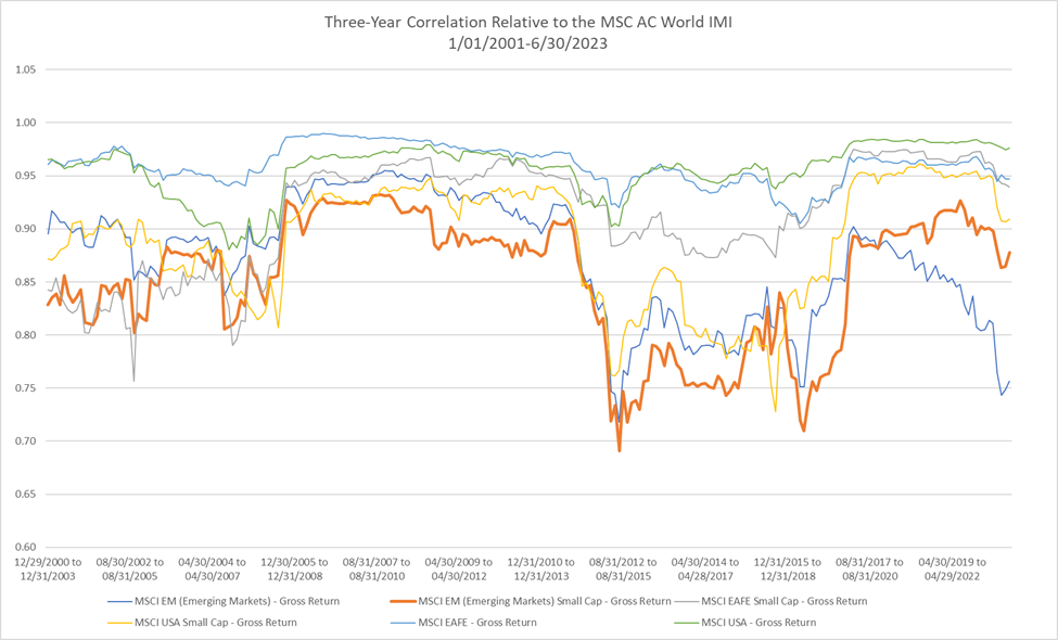
Much has been written about how the emerging markets equity asset class can be a good diversifier to other equity asset classes. This also holds true for emerging markets small-cap equity. The simplest way to confirm this is to view the correlation of the asset class versus other equity asset classes. We looked at rolling 36-month correlations using monthly returns for various MSCI indexes (to represent various equity asset classes) relative to the MSCI AC World IMI, an index that constitutes large-, mid-, and small-cap companies across 23 developed markets and 24 emerging markets. Since the common inception in 2001 of the indexes shown, the MSCI Emerging Markets Small Cap Index as a proxy for the emerging markets small-cap equity asset class has consistently been among the lowest correlated index relative to the MSCI AC World IMI.
Source: FactSet; Returns for the MSCI Emerging Markets prior to June 2007 are back-tested performance and do not reflect actual index performance. Back-tested index performance was calculated retroactively to show how the index might have performed and may be materially different than actual results would have been.
However, for the most recent three-year period, the lowest correlation has been between the MSCI Emerging Markets Index to the MSCI AC World IMI. To what can we attribute this sudden dip? The primary reason is the large weighting that China has in the MSCI Emerging Markets Index versus the MSCI Emerging Markets Small Cap Index. The following table shows each index’s average weight to China and overall index return all for the three years ending June 30, 2023.
Three Years as of 6/30/23
Average Weight to China
Overall Index Cumulative Return (Net)
MSCI Emerging Markets Small Cap Index
11.08%
47.06%
MSCI Emerging Markets Index
39.03%
7.12%
Source: FactSet
While the performance of Chinese stocks in the MSCI Emerging Markets Small Cap Index was worse on an absolute basis relative to the overall MSCI Emerging Markets Index, the lower weighting to China mitigated the negative effect to the overall performance of the MSCI Emerging Markets Small Cap Index. The MSCI Emerging Markets Index’s 3.5 times higher average weight to China had a significant negative effect on performance. This tells us that indeed, the MSCI Emerging Markets Index has lower correlation in the most recent period, but that correlation has come at a cost.
Viewing correlations for the MSCI Emerging Markets Small Cap Index versus various representative non-equity indexes shows that correlations are also low for this asset class relative to non-equity asset classes. And while some correlations have nominally crept up in recent years, the long-term correlations of the MSCI Emerging Markets Small Cap Index have remained low for longer time periods.
Correlation Relative to MSCI Emerging Markets Small Cap Index (Using Daily Returns) as of 06/30/2023
Asset Class
Index Representative
3 Year
5 Year
10 Year
US Broad Fixed Income
Bloomberg Barclays US Aggregate
0.03
0.01
-0.01
US High Yield Fixed Income
Bloomberg Barclays US High Yield – Corporate
0.50
0.62
0.58
US Real Estate
MSCI US REIT INDEX – Gross Return
0.22
0.38
0.33
Commodities
S&P GSCI Total Return
0.24
0.29
0.26
Source: FactSet
Lower correlations may also be attributed to larger differences in cyclical versus defensive sectors, which can – and have – driven differences in returns even within emerging markets. Comparing the sector weights of the MSCI Emerging Markets Small Cap Index versus the MSCI Emerging Markets Large Cap Index shows these stark differences. In the table below, cyclical sectors (Communication Services, Consumer Discretionary, Financials, Industrials, Information Technology, and Materials) had an average weight difference of 7.32%, while defensive sectors (Consumer Staples, Energy, Health Care, Real Estate, and Utilities) had an average weight difference of 3.10%. As these differences persist, correlations may remain lower particularly during different economic regimes, which provides good diversification opportunities for emerging markets small-cap.
Sector Weights (%) As of 6/30/2023
MSCI Emerging Markets Small Cap Index
MSCI Emerging Markets Large Cap Index
Absolute Difference
Industrials
16.78
4.97
11.81
Financials
10.91
22.28
-11.37
Communication Services
4.02
10.81
-6.79
Materials
13.95
7.49
6.46
Health Care
8.89
2.79
6.10
Information Technology
17.09
22.49
-5.40
Real Estate
6.14
1.35
4.78
Energy
1.77
5.30
-3.53
Consumer Discretionary
11.10
13.20
-2.10
Utilities
3.19
2.28
0.91
Consumer Staples
6.12
5.93
0.19
Source: FactSet
As seen above with China, another potential contributor to lower correlations and drivers to return within emerging markets small-cap is the difference in country allocations. An examination of country weights of the MSCI Emerging Markets Index versus the MSCI Emerging Markets Small Cap Index shows some stark differences.
Country Weights (%) as of 06/30/2023
Country
MSCI Emerging Markets Small Cap Index
MSCI Emerging Markets Index
Absolute Difference
China
8.07
29.55
21.48
India
24.23
14.63
9.61
Taiwan
21.81
15.60
6.21
Korea
14.99
12.30
2.69
Thailand
3.22
1.92
1.30
Malaysia
2.37
1.33
1.04
Turkey
1.48
0.55
0.92
Mexico
2.37
2.80
0.43
South Africa
2.78
3.21
0.43
Saudi Arabia
3.80
4.22
0.43
Chile
0.89
0.54
0.35
United Arab Emirates
0.96
1.30
0.34
Philippines
0.98
0.65
0.33
Poland
1.12
0.85
0.27
Peru
—
0.26
0.26
Brazil
5.80
5.54
0.26
Kuwait
1.05
0.83
0.22
Hungary
0.04
0.24
0.20
Indonesia
2.19
2.00
0.19
Greece
0.64
0.45
0.19
Egypt
0.26
0.08
0.18
Czech Republic
0.06
0.15
0.10
Qatar
0.83
0.90
0.07
Columbia
0.10
0.10
0.00
Source: FactSet
As with China, the other top two largest country weight differences – India and Taiwan – have had an outsized effect on performance (and thus correlations). In the last three years, India has had a staggering 122.58% return in the MSCI Emerging Markets Small-Cap versus the MSCI Emerging Markets India return of 72.68%. The difference in weightings have also affected performance and correlation with the MSCI Emerging Markets Small-Cap Index having nearly 10% more in India relative to the MSCI Emerging Markets Index. And while the returns for Taiwanese stocks were similar between the two Indexes, the large positive return and relative overweighting in the MSCI Emerging Markets Small-Cap Index had a positive effect. Like the differences in sectors, as these differences in country weights persist correlations may remain lower, and broader diversification opportunities across countries may continue to exist for emerging markets small-cap.
Active Management in Emerging Markets Small-Cap
The argument on whether to pursue an active versus passive approach in equity strategies has been long debated with strong proponents on each side. Each side has put forth compelling considerations. However, we believe that in the case of the emerging markets small-cap, active management has an edge over passive management. Historical evidence has shown that active management in emerging markets small-cap equity tends to well outperform a common benchmark, which is not always the case for other asset classes.
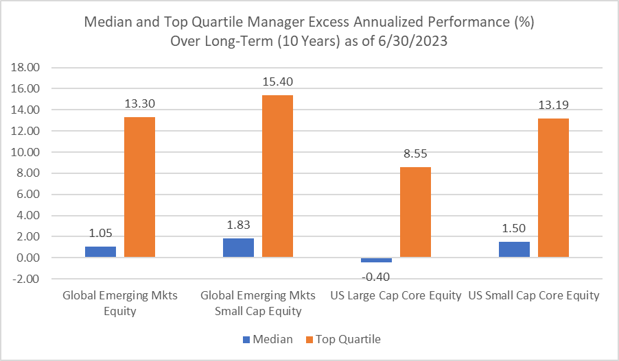
In the updated chart below, we show the excess annualized gross return over the long-term (10 years) of the median and top quartile institutional manager in four equity universes from the eVestment database: Global Emerging Markets Equity, and Global Emerging Markets Small Cap Equity, US Large Cap Core Equity, US Small Cap Core Equity against a common benchmark for each universe.
Source: eVestment, Bridgeway analysis; the eVestment universe median and top quartile calculation is using the default reporting method and default vehicle for all universe constituents to determine the median for each universe. The benchmark used for the Global Emerging Mkts Equity manager is the MSCI Emerging Markets Index Net; the benchmark used for the Global Emerging Mkts Small Cap Equity manager is the MSCI Emerging Markets Small Cap Index Net; the benchmark used for the US Large Cap Core Equity manager is the Russell 1000 Index Total Return; and the benchmark used for the US Small Cap Core Equity manager is the Russell 2000 Index Total Return.
Over this long-term period, the median Global Emerging Markets Small Cap Equity manager provides the highest excess performance of any of the other median managers shown relative to their benchmarks. Narrowing it down to the top quartile in each universe shows a similar pattern: the Global Emerging Markets Small Cap Equity manager has the highest excess performance of any of the other top quartile managers shown relative to their benchmarks. We believe this is strong evidence that persistent excess return in emerging market small-cap equity can be achieved with an active approach to management.
Is Emerging Markets Small-Cap an Attractive Asset Class Now?
More than two years has passed since we launched our own emerging markets small-cap strategy. At the time of launch, we believed it was an attractive asset class and continue to believe so now. However, a strong caveat: the question of whether to invest in any asset class at a particular time very often hints at market timing, something we do not suggest attempting. Even the most sophisticated investors would need to get the timing right multiple times for each asset class if a market-timing approach were implemented.
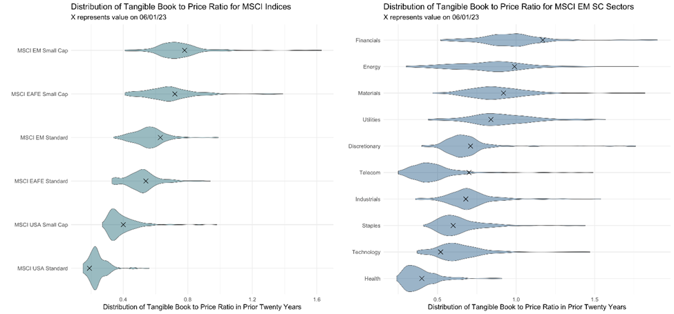
Nevertheless, asking the question of whether emerging markets small-cap is an attractive asset class now can be informative and assist with understanding how the asset class fits into an overall asset allocation. To do this, we plotted the distribution of tangible book-to-price ratios for the past 20 years and noted where each index stands as of June 1, 2023.
Source: FactSet, Bridgeway analysis
As the chart above on the left demonstrates, the MSCI Emerging Markets Small Cap Index generally has a distribution of book-to price ratios that are higher (meaning it represents a stronger value profile) than the other indexes represented. Further, within that distribution, the MSCI Emerging Markets Small Cap Index is currently cheap relative to its own history, making it an attractive opportunity for value investors. The chart on the right decomposes the MSCI Emerging Markets Small Cap Index into sectors and similarly plots the book-to-price ratios for each over the past 20 years. Except for the outlier of Information Technology, the chart shows that within MSCI Emerging Markets Small Cap Index, each sector is currently cheap relative to its own history demonstrating that the value opportunities in this space are broad based and not just driven by one particular sector.
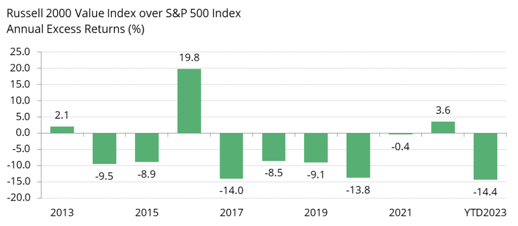
For almost ten years, cheap stocks have lagged expensive stocks in terms of performance. This is a rare occurrence in the history of the market. Moreover, this trend is not limited to one region or country, but has affected the whole world. Therefore, we believe that emerging market small-cap stocks are poised to outperform, as they offer a great opportunity for value-focused investors. These stocks are currently trading at very attractive valuations, both compared to other global equities and to their own historical averages. Investors who are looking for the best bargains in the market should not miss the chance to invest in emerging markets small-cap stocks now.
Investing Quantitatively and Managing Capacity in Emerging Markets Small-Cap
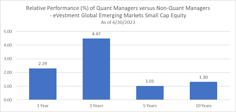
In our 2021 piece, we discussed why a quantitative approach has some advantages over a non-quantitative approach. In summary, because a quantitative approach relies on data and can use modern programming and statistical analysis to evaluate companies, quantitative investment managers can cover the large number of names in the universe more quickly and efficiently than a non-quantitative manager. Further, because a quantitative approach allows an investment manager to cover all the names in the universe on a daily basis, there may be more potential opportunities for a quantitative investment manager than a non-quantitative manager may ever discover. Reviewing the data in eVestment appears to back up this hypothesis.
Source: eVestment, Bridgeway analysis; for each period, the average return of managers with a non-quantitative investment approach is subtracted from the average return of managers with a quantitative investment approach. The returns used are for the default reporting method and default vehicle for all universe constituents to calculate the average.
Over the trailing, 1-, 3-, 5-, and 10-year periods ending June 30, 2023, the average return for managers with a quantitative approach have outperformed their non-quantitative peers in the range of 1.01 – 4.47% annualized.
However, a good performing strategy is only good as long as it sticks to its mandate, which is why managing capacity is so important. At Bridgeway, we believe in doing what is best for the long-term interests of existing investors. This means that in asset classes that are capacity constrained, we will close at responsible levels in order to maintain the integrity of the investment process for our existing investors. Bridgeway has a history of closing strategies early to protect the process and existing investors, even when it means turning down large amounts of assets. In fact, in one of our most capacity-constrained strategies, we have been closed to new investors for more than a decade.
Bridgeway’s experience in managing assets in capacity-constrained asset classes can help successfully guide our experience in the emerging markets small-cap universe. Additionally, Bridgeway’s international equity team, led by our Co-CIO and Head of International Equity, Jacob Pozharny, PhD, has more than 25 years managing non-US equity strategies, including in capacity constrained asset classes. Along with the support and expertise of the entire investment management team at Bridgeway, this creates an experience in which our investors can be confident that we have their long-term interests in mind and that our investment philosophy and approach maintain integrity.
Bridgeway in Emerging Markets Small-Cap
In our last piece on “Why Emerging Markets Small-Cap?” we noted our innovative approach incorporating intangibles in our own Emerging Markets Small-Cap strategy. To summarize, we believe that equity price changes are driven primarily by financial fundamentals over the long run. However, as companies increasingly rely on intangible assets to drive business, we have seen these intangible assets displace traditional tangible, physical assets affecting financial statements. Based on our research, we believe that categorizing companies based on their Intangible Capital Intensity (ICI) has the potential to improve stock selection by using the most relevant metrics, particularly in non-US markets. Our framework for ICI is determined at the industry level, with high ICI industries having higher levels of intangible investment (e.g., pharmaceuticals, software, telecom services, media, etc.) while low ICI industries have lower levels of intangible investment (e.g., utilities, materials, capital goods, real estate, etc.). We then contextually apply factors like value, quality, sentiment, and trend to shape stock selection.
Bridgeway further differentiates our approach to investing in emerging markets small-cap stocks through portfolio construction innovation. We use a unique approach to invest in emerging markets small-cap stocks that focuses on both picking the best stocks and building the best portfolio, emphasizing both equally.
Our portfolio construction is driven by sizing index-relative exposures using an innovative technique we call Active Share Proportionality rather than classical mean-variance optimization. Our research indicates that off-the-shelf optimizers that are based on mean-variance optimization depend on the stability of a covariance matrix and use too much turnover to adapt the portfolio to noisy volatility estimates. Unlike most investors who rely on these standard tools that adjust the portfolio based on how stocks move together, we construct our portfolio in a differentiated manner. Our method of Active Share Proportionality allows us to size our systemic risks directly based on how much they proportionally differ from the index, rather than how much stocks vary with each other. This way, we seek to avoid the problems of using unreliable and changing estimates of stock correlations, which often lead to unnecessary trading and higher costs. By not requiring a covariance matrix estimate, our portfolio construction technique reduces turnover requirements and transaction costs, thus turnover exists primarily to express stock preferences rather than adapt to covariance noise.
This technique is geared to source active return from idiosyncratic elements rather than systematic risks. Our method helps us to reduce the impact of market-wide factors, such as country, sector, size, and Beta, and to increase the contribution of stock-specific factors, such as company fundamentals, growth, and sentiment, to our performance. By doing this, we aim to generate more consistent and diversified returns from our stock selection and mute systematic exposures to improve the risk-adjusted excess return of our portfolio.
Conclusion
We have demonstrated some convincing reasons to invest in emerging markets small-cap equity including an attractive value profile and diversification opportunity. Most convincing, though, may be the emerging markets share of global GDP and global GDP growth. Currently, emerging markets countries “account for 50% of Global GDP and 66% of global GDP growth in the past 10 years (2012-2022).”[1] With this kind of representation globally, it is likely that most investors are underallocated to emerging markets. This evidence should compel investors to look at emerging markets more closely and potentially as a larger portion of an overall allocation.
With the Bridgeway Emerging Markets Small-Cap strategy, we combine an attractive asset class with established experience, expertise, and a reputation for maintaining integrity by managing capacity responsibly. The Bridgeway Emerging Markets Small-Cap strategy lies squarely at the intersection of our investment expertise and how we can best serve our clients. We are confident we can offer a unique strategy in emerging markets small-cap equity with high conviction in our investment philosophy and process.
The opinions expressed here are exclusively those of Bridgeway Capital Management (“Bridgeway”). Information provided herein is educational in nature and for informational purposes only and should not be considered investment, legal, or tax advice.
Past performance is not indicative of future results.
Investing involves risk, including possible loss of principal. In addition, market turbulence and reduced liquidity in the markets may negatively affect many issuers, which could adversely affect the strategy. Value stocks as a group may be out of favor at times and underperform the overall equity market for long periods while the market concentrates on other types of stocks, such as “growth” stocks. Emerging markets are those countries that are classified by MSCI as emerging markets and generally consist of those countries with securities markets that are less sophisticated than more developed markets in terms of participation, analyst coverage, liquidity, and regulation. These are markets that have yet to reach a level of maturity associated with developed foreign stock markets, especially in terms of participation by investors. These risks are in addition to the usual risks inherent in U.S. investments. There is the possibility of expropriation, nationalization, or confiscatory taxation, taxation of income earned in foreign nations or other taxes imposed with respect to investments in foreign nations, foreign exchange control (which may include suspension of the ability to transfer currency from a given country), default in foreign government securities, political or social instability, or diplomatic developments which could affect investments in securities of issuers in those nations. The government and economies of emerging markets feature greater instability than those of more developed countries. Such investments tend to fluctuate in price more widely and to be less liquid than other foreign investments. Investments in small companies generally carry greater risk than is customarily associated with larger companies. This additional risk is attributable to a number of reasons, including the relatively limited financial resources that are typically available to small companies, and the fact that small companies often have comparatively limited product lines. In addition, the stock of small companies tends to be more volatile and less liquid than the stock of large companies, particularly in the short term and particularly in the early stages of an economic or market downturn.
Diversification neither assures a profit nor guarantees against loss in a declining market.
The Bloomberg Barclays US Aggregate Bond Index is a broad-based flagship benchmark that measures the investment grade, US dollar-denominated, fixed-rate taxable bond market. The index includes Treasuries, government-related and corporate securities, MBS (agency fixed-rate and hybrid ARM pass-throughs), ABS, and CMBS (agency and nonagency). Provided the necessary inclusion rules are met, US Aggregate-eligible securities also contribute to the multicurrency Global Aggregate Index and the US Universal Index, which includes high yield and emerging markets debt.
The Bloomberg Barclays US Corporate High Yield Bond Index measures the USD-denominated, high-yield, fixed-rate corporate bond market. Securities are classified as high yield if the middle rating of Moody’s, Fitch and S&P is Ba1/BB+/BB+ or below. Bonds from issuers with an emerging markets country of risk, based on the indices’ EM country definition, are excluded. The US Corporate High Yield Index is a component of the US Universal and Global High Yield Indices.
The MSCI EAFE Index is an equity index which captures large and mid cap representation across 21 Developed Markets countries around the world, excluding the US and Canada. With 874 constituents, the index covers approximately 85% of the free float-adjusted market capitalization in each country.
The MSCI EAFE Small Cap Index is an equity index which captures small cap representation across Developed Markets countries around the world, excluding the US and Canada. With 2,354 constituents, the index covers approximately 14% of the free float-adjusted market capitalization in each country.
The MSCI Emerging Markets Index captures large and mid cap representation across 27 Emerging Markets (EM) countries. With 1,381 constituents, the index covers approximately 85% of the free float-adjusted market capitalization in each country. Net total return represents reinvested dividends after the deduction of withholding taxes, using a tax rate applicable to non-resident institutional investors who do not benefit from double taxation treaties.
The MSCI Emerging Markets Small Cap Index includes small cap representation across 27 Emerging Markets countries. With 1,692 constituents, the index covers approximately 14% of the free float-adjusted market capitalization in each country. The small cap segment tends to capture more local economic and sector characteristics relative to larger Emerging Markets capitalization segments. Net total return represents reinvested dividends after the deduction of withholding taxes, using a tax rate applicable to non-resident institutional investors who do not benefit from double taxation treaties. The MSCI US REIT Index is a free float-adjusted market capitalization weighted index that is comprised of equity Real Estate Investment Trusts (REITs). The index is based on the MSCI USA Investable Market Index (IMI), its parent index, which captures the large, mid and small cap segments of the USA market. With 137 constituents, it represents about 99% of the US REIT universe and securities are classified under the Equity REITs Industry (under the Real Estate Sector) according to the Global Industry Classification Standard (GICS®), have core real estate exposure (i.e., only selected Specialized REITs are eligible) and carry REIT tax status.
The MSCI USA Index is designed to measure the performance of the large and mid cap segments of the US market. With 620 constituents, the index covers approximately 85% of the free float-adjusted market capitalization in the US.
The MSCI USA Small Cap Index is designed to measure the performance of the small cap segment of the US equity market. With 1,741 constituents, the index represents approximately 14% of the free float-adjusted market capitalization in the US.
The S&P GSCI index measures commodity market performance through futures. The S&P GSCI is weighted by world production and comprises the physical commodities that have active, liquid futures markets. There is no limit on the number of commodities that may be included in the S&P GSCI; any commodity whose contract satisfies the eligibility criteria and the other conditions specified in this methodology are included.
The Russell 1000 Index includes approximately 1,000 of the largest companies in the US equity universe. It includes approximately 1,000 of the largest securities based on a combination of their market cap and current index membership. The Russell 1000 Index is constructed to provide a comprehensive and unbiased barometer for the large-cap segment and is completely reconstituted annually to ensure new and growing equities are included.
The Russell 2000 Index measures the performance of the small-cap segment of the US equity universe. The Russell 2000 Index includes approximately 2,000 of the smallest securities based on a combination of their market cap and current index membership. The Russell 2000 is constructed to provide a comprehensive and unbiased small-cap barometer and is completely reconstituted annually to ensure larger stocks do not distort the performance and characteristics of the true small-cap opportunity set.
One cannot invest directly in an index. Index returns do not reflect fees, expenses or trading costs associated with an actively managed portfolio.
Exchange-traded funds (ETFs) have seen tremendous growth since their initial launch in 1993. As with mutual funds, they hold a collection of securities. Unlike mutual funds, which trade at the end of the day at net asset value (NAV), ETFs trade throughout the day on exchanges like individual stocks, but at a premium or discount to the NAV of the underlying securities.
Because ETFs trade throughout the day at prices which differ from the underlying value of the securities they hold, greater care should be taken to achieve best execution when trading them. In this paper, we provide a brief guide to trading ETFs. These points should be useful to both individual investors and advisors executing smaller trades on their own, and for larger institutional investors and advisors with access to institutional quality trading desks.
Liquidity. While ETFs trade on an exchange, their trading is different than individual stocks. Transactions for ETFs occur on both a primary and secondary market. The primary market is where Authorized Participants (APs) create or redeem shares in an ETF. These transactions are typically done via in-kind transfers and are the source of the increased tax efficiencies of ETFs. The liquidity in the primary market for APs is directly influenced by the liquidity of the underlying fund holdings. The secondary market is where individual trades of the ETF occur. The volume quoted for an ETF reflects this secondary market activity and doesn’t account for the primary market liquidity. An ETF with typically low secondary market volume can still have large transactions occur within the spread based on the primary market liquidity. Thus, for most ETFs, liquidity available is beyond what is quoted in the secondary market.
Avoid market open and close. Similar to individual stocks, prices tend to be more volatile around the open and close of the market, which can lead to wider bid-ask spreads in ETFs. Since the spread of an ETF reflects the spreads of the securities it holds, the price you trade at near the market open and close may be further from the NAV of those underlying securities. A good rule of thumb is to trade between 10:00 AM and 3:30 PM Eastern Time, avoiding the first and last 30 minutes of the trading day.
Use limit orders when possible. Market orders are certainly convenient, as you are guaranteed certainty of execution. But if there is insufficient interest on the other side of the trade for a market order, you can exhaust the limit order book and pay a substantial spread to fair value. Instead, place limit orders with your brokers, adjusting as needed for market moves. This is especially true for larger orders and at times of lower liquidity. While market orders demand liquidity, limit orders provide liquidity and thus can potentially take advantage of the spread.
Consider your overall trading. When cash is being invested or withdrawn, just a single ETF may be traded. But other times, such as during rebalancing or tax loss harvesting, multiple ETFs and mutual funds may be bought and sold. In this case, consider the timing and interaction of the trades to minimize slippage from market movement.
Make use of your advisory firm’s trading desk. As trades get larger and more complicated, selecting between various techniques and executing them well may appear daunting. But, many financial advisors are affiliated with a larger firm that provides trading services. The trading desk can aggregate the trades of multiple advisors to get a better understanding of liquidity and access methods available with scale. The trading desk has the time, experience, and tools to focus on the best methods for executing your ETF trades, allowing advisors to focus on what they do best. If you have access to a centralized trade execution team, they will be the preferred solution when trading ETFs. For larger orders, consider the following techniques:
Use an RFQ with your broker for large orders. If you are placing a large order that exceeds a creation unit size (this varies by fund but can be 25,000 shares or more), consider getting in touch with the ETF trading desk you work with and receive a request for quote (RFQ). With an RFQ, an institutional investor solicits bids from several brokers for a larger trade to get better pricing.
Place a direct creation/redemption with your broker. Some brokers are also APs. For a sufficiently large order, they can place direct creations and redemptions. Much like mutual funds, the ETF price will be market at closing NAV. This may result in lower costs, depending on the fees charged by the broker/AP.
Utilize your custodian’s ETF desk. Many custodians maintain ETF trading desks. With their expertise, they can often uncover hidden liquidity and arrange trades to get great pricing and execution. Contact your custodian trading desk to request automatic review of any large market order, typically over 10,000 shares. Many custodians offer to watch your trading master for large orders. Once they identify the order, they will trade them for best execution.
ETFs have some notable advantages, which have led to their tremendous growth. The use of APs allows for the avoidance of capital gains within the fund. The transaction costs of cash flows into and out of the ETF are borne by those trading and not the ETF itself. But this also means that one must be careful when trading ETFs, to minimize slippage and achieve best execution. In this paper, we have provided tips that should be helpful when trading ETFs for the benefit of you and those you serve. After all, the purpose of trading ETFs is to invest in ETFs and realize the benefits they offer.
Andrew L. Berkin, PhD Head of Research Bridgeway Capital Management
Andrew Berkin, PhD, is head of research and oversees the development and implementation of Bridgeway’s statistically driven, evidence-based investment strategies. He also produces thought leadership material for clients and prospects as well as for external publications. Andrew joined Bridgeway in 2013. Prior to joining Bridgeway, Andrew was co-chief investment officer and director of research for Vericimetry Advisors. He previously was a senior member and director of the quantitative research group at First Quadrant, where he spent 14 years in a variety of responsibilities, including the development and implementation of stock selection models in both taxable and tax-exempt portfolios. Andrew has published numerous research articles on quantitative investing in peer-reviewed journals and co-authored two books. He is a reviewer for the Financial Analysts Journal and served two terms on its editorial board. Andrew earned his BS with honors in Physics from the California Institute of Technology and a PhD of Philosophy in Physics from the University of Texas, where he concentrated his studies in general relativity and astrophysics.
Ben Lanning Director of Portfolio Management Buckingham Strategic Wealth
When he joined Buckingham Strategic Wealth in 2005, Ben Lanning already knew he loved the investment business. What he discovered when he came to Buckingham was that he’d found the perfect place to do it. Ben serves as the director of portfolio management, working with Buckingham’s dedicated team of portfolio managers to monitor clients’ portfolios and ensure appropriate allocations. Previously, he was a relationship director and director of trading operations, working with both advisors and with clients to make sense of the technical, research-based philosophy behind the firm’s fixed income and equity trading approach. Ben started with the firm as an equity trader and fell in love with client-first, bottom line second attitude his colleagues espoused. Knowing he could make recommendations without bias, that his colleagues spent their days collaborating on how best to solve a problem for a client and being a part of the evidence-based movement keeps Ben excited and engaged. Prior to joining Buckingham, Ben was a senior trader with Raymond James. He is a graduate of St. Petersburg College and Eckerd College. He and his wife, Natalie, live in St. Louis with their two children.
Christine Wang, CFA, CPA Portfolio Manager Bridgeway Capital Management
Christine’s responsibilities include portfolio management, investment research, and statistical modeling. Prior to joining Bridgeway, she worked in public accounting with a focus on energy trading and risk management. Christine holds an MS in Accounting from the University of Virginia and a BA in Sociology and Managerial Studies from Rice University. She is a CFA charterholder and is licensed as a Certified Public Accountant in Texas. She participated in Bridgeway’s service trip to Peru. On Bridgeway’s service trips to Honduras and El Salvador, she helped build water wells with Living Water International.
DISCLOSURE
The opinions expressed here are exclusively those of Andrew L. Berkin, Ben Lanning, and Christine Wang. Information provided herein is educational in nature and for informational purposes only and should not be considered investment, legal, or tax advice.
Investing involves risk, including possible loss of principal. In addition, market turbulence and reduced liquidity in the markets may negatively affect many issuers, which could have an adverse effect on such investments.
Waiting on the World to Change – Small-Cap Value Investors
Small-cap value stocks have lagged the large-cap S&P 500 by significant amounts to start 2023.
This dispersion of returns has led to small-cap value stocks being extremely cheap compared to the S&P 500.
Combined with the narrowness of returns within the S&P 500, such conditions have historically provided an opportunity for strong reversion, with small-cap value stocks outperforming.
Waiting for the World to Change
As small-cap value investors, sometimes it feels like you are just Waiting on the World to Change. The Russell 2000 Value Index lagged the S&P 500 Index of large US companies by a significant margin four years in a row from 2017 through 2020. The Russell 2000 Value staged a comeback in early 2021 (see our piece Room to Run), offering glimpses that we had turned a corner, but 2023 has reverted to the same chorus. It sometimes feels like we’re stuck with a broken record.
Source: Bloomberg
We at Bridgeway are firm believers in the small and value factors. These drivers of returns are integral parts of our investment process. Using the full history currently available from the Ken French data library (July 1926 – May 2023), we find small-cap value stocks have returned 14.1% annually, compared to 10.0% for the broad market. Not only do these factors historically provide a return premium, but they also meet our criteria of being persistent, pervasive, robust, investable, and intuitive. Furthermore, they provide useful diversification to the overall portfolio. (See the book Your Complete Guide to Factor-Based Investing by Andrew Berkin and Larry Swedroe for further discussion.)
Given small-cap value’s recent performance, where do we stand right now?
Using the standard academic definition of valuation, book-to-market (BtM), we can put into perspective where we are relative to history. The blue line in the chart below shows the ratio of median BtM for the Russell 2000 Value Index to median BtM for the S&P 500. The solid orange line shows the median ratio for the entire history of the Russell 2000 Value from 1978- June 2023. Ratios above this line signal that small-cap value stocks are cheaper than their historical average.
Median BtM Ratios Relative to S&P500 For the Period Ending 6/30/23
Source: Compustat, Bridgeway calculations
The first big spike when the Russell 2000 Value was cheaper than the S&P 500 was the dot.com era. Investors did Party Like It’s 1999, favoring high-flying growth stocks over value stocks. Valuations then reverted to the median (yielding five years of double-digit outperformance of the Russell 2000 Value vs. the S&P 500). The 2010s saw valuations creep back up, culminating in a new peak in 2020 of how cheap small-cap value had gotten relative to the S&P500. That reversed dramatically (and quickly) in 2021, bringing relative valuations down but still higher than historical levels. The relative underperformance of small-cap value in 2023 has stretched the ratio again, getting us close to, but not yet at the prior peak. This potentially sets the stage for a future reversal with strong small-cap value outperformance.
In the recent period, small-cap stocks, represented by the Russell 2000, have faced a similar relationship to the S&P 500 (grey line) as the Russell 2000 Value, becoming far cheaper than their median (yellow line). Small caps in general are now even cheaper than the historical median Russell 2000 Value to S&P 500 ratio.
So why stick to small-caps and value in particular? For one, the rally in the S&P 500 has been concentrated in a few stocks. While this is not new (see our piece on the Nifty Fifty), it does mean the rally has lacked breadth. The equal weight S&P 500 lagged the index by almost 10% to begin 2023. That’s in the worst 2% of six-month periods going back to 1990 when Bloomberg data starts. Small-cap value is incredibly cheap right now and while things could get worse before they get better, we encourage you to Don’t Stop Believin’. Stick with your allocation and rebalance. That would be music to our ears.
The opinions expressed here are exclusively those of Bridgeway Capital Management (“Bridgeway”). Information provided herein is educational in nature and for informational purposes only and should not be considered investment, legal, or tax advice.
Past performance is not indicative of future results.
Investing involves risk, including possible loss of principal. In addition, market turbulence and reduced liquidity in the markets may negatively affect many issuers, which could adversely affect client accounts. Value stocks as a group may be out of favor at times and underperform the overall equity market for long periods while the market concentrates on other types of stocks, such as “growth” stocks.
Diversification neither assures a profit nor guarantees against loss in a declining market.
The S&P 500 Index is a broad-based, unmanaged measurement of changes in stock market conditions based on the average of 500 widely held common stocks.
The Russell 2000 Index is an unmanaged, market value-weighted index, which measures the performance of the 2,000 companies that are between the 1,000th and 3,000th largest in the market. The Russell 2000 Value Index measures the performance of those Russell 2000 companies with lower price-to-book ratios and lower forecasted growth values.
One cannot invest directly in an index. Index returns do not reflect fees, expenses, or trading costs associated with an actively managed portfolio.
Emerging Markets Small-Cap Investment Landscape: August 2021
As we continue to monitor economic and market trends in emerging markets (EM), we find that the Price-to-Book – Return on Equity (PB-ROE)[1] analysis we described in our last update offers a flexible methodology for applying different lenses to the EM investment landscape.
Our last analysis used the PB-ROE analysis to examine how cheap or expensive different EM countries were relative to their level of profitability. In this update, we’re comparing valuations and profitability among major industries in the EM small-cap universe. To provide additional context that’s important to many investors, we’ve also applied a layer of Environmental, Social, and Governance (ESG) analysis to examine the potential relationships between valuation, profitability, and ESG considerations.
The chart below highlights conditions in the EM small-cap landscape as of June 30, 2021.
The y-axis plots each industry’s median book yield, placing cheaper industries higher on the chart.
The x-axis plots each industry’s median return on equity, placing more profitable industries farther to the right.
Industries are color-coded according to their median ESG scores based on MSCI ESG ratings. Industries in orange have the lowest median ESG scores, while industries in blue have the highest.
Source: FactSet, MSCI, and Bridgeway
More profitable industries typically command a higher valuation. We expect that the cross-section of industry Book Yield and ROE medians to be negatively correlated as more profitable industries are more expensive while less profitable industries are less expensive. This chart uncovers investment opportunities in the outliers – industries that don’t conform to these expectations. So what does this PB-ROE scatter chart tell us about EM small-cap industries?
Lower profitability or valuation
Consumer Services and Transportation currently have the lowest profitability—and also look quite expensive given those low levels of profits. We see the impact of COVID-19 on those two industries, which were hit particularly hard by lockdowns.
Banks and Real Estate companies in the EM small-cap universe are viewed as risky by investors and are valued cheaply considering their ROEs. They certainly don’t conform to our PB-ROE expectations because of the economic pressures that COVID-19 has placed on these industries. For example, investors may see bank loans and real estate rents as at-risk as segments of the economy as borrowers may not be able to pay mortgage and interest payments. Further, global COVID-19 policies have placed significant pressures on commercial real estate properties. Our PB-ROE model see these industries as interesting opportunities as market expectations stabilize. We will be monitoring their profitability levels and earnings forecasts closely to determine if the current valuations and investor reactions are overdone.
Higher profitability or valuation
At the far right of the chart above, we see industries that benefited from the pandemic: Household and Personal Products, Commercial and Professional Services, Software, and Semiconductors enjoyed higher demand and higher profits as consumers stocked up on household goods and electronic devices during lockdowns. At the same time, valuations have risen, making these industries relatively expensive.
ESG Considerations
Given the rising interest in sustainability and ESG strategies, understanding how different industries perform on ESG metrics can be another important consideration for EM investors. In the bar chart to the left of the PB-ROE analysis above, we’ve ranked industries by median ESG score based on MSCI ESG ratings. MSCI’s methodology is one of the leading industry frameworks for determining a company’s resilience to long-term financially relevant ESG risks. More specifically, MSCI ESG scores measure exposure to ESG risks and opportunities at the industry level. Each industry is evaluated on the three pillars – Environmental, Social, and Governance – which comprise 10 separate themes. Each theme has multiple Key Issues that may or may not be relevant to a company’s specific industry. Company specific MSCI ESG ratings are a weighted average of the scores on the Key Issues and are normalized relative to the compay’s industry peers. In the bar chart, the lowest-scoring industries are at the top, while the highest-scoring industries are at the bottom:
Telecommunication Services and Utilities currently have the highest overall median ESG ratings in the emerging markets small-cap universe.
Household and Personal Products and Semiconductors/Semiconductor equipment have the lowest overall ESG ratings. Household and Personal Products historically (and currently) have a particularly low median score on the Environment pillar of the MSCI ESG scoring methodology, while the semiconductor industry has a particularly low median Governance score.
As with other metrics, this is a snapshot in time: industry median ESG scores and their rankings change over time. But for EM small-cap investors interested in incorporating ESG into their portfolios, this data provides additional context about conditions in the EM small-cap universe. Bridgeway investment professionals have extensive experience building ESG-aware, non-US equity portfolios that seek a strong risk-adjusted return profile while simultaneously seek to improve the ESG profile across industries and countries using our proprietary Active Share Proportionality portfolio construction techniques.
[1] PB-ROE are financial measures referring to the price-to-book (PB) ratio and return on equity (ROE) of a company.
DISCLOSURE
The opinions expressed here are exclusively those of Bridgeway Capital Management (“Bridgeway”). Information provided herein is educational in nature and for informational purposes only and should not be considered investment, legal, or tax advice.
Past performance is not indicative of future results.
Investing involves risk, including possible loss of principal. In addition, market turbulence and reduced liquidity in the markets may negatively affect many issuers, which could adversely affect client accounts. Value stocks as a group may be out of favor at times and underperform the overall equity market for long periods while the market concentrates on other types of stocks, such as “growth” stocks. Emerging markets are those countries that are classified by MSCI as emerging markets and generally consist of those countries with securities markets that are less sophisticated than more developed markets in terms of participation, analyst coverage, liquidity, and regulation. These are markets that have yet to reach a level of maturity associated with developed foreign stock markets, especially in terms of participation by investors. These risks are in addition to the usual risks inherent in U.S. investments. There is the possibility of expropriation, nationalization, or confiscatory taxation, taxation of income earned in foreign nations or other taxes imposed with respect to investments in foreign nations, foreign exchange control (which may include suspension of the ability to transfer currency from a given country), default in foreign government securities, political or social instability, or diplomatic developments which could affect investments in securities of issuers in those nations. The government and economies of emerging markets feature greater instability than those of more developed countries. Such investments tend to fluctuate in price more widely and to be less liquid than other foreign investments. Investments in small companies generally carry greater risk than is customarily associated with larger companies. This additional risk is attributable to a number of reasons, including the relatively limited financial resources that are typically available to small companies, and the fact that small companies often have comparatively limited product lines. In addition, the stock of small companies tends to be more volatile and less liquid than the stock of large companies, particularly in the short term and particularly in the early stages of an economic or market downturn.
Diversification neither assures a profit nor guarantees against loss in a declining market.
The MSCI Emerging Markets Small Cap Index includes small cap representation across 27 Emerging Markets countries. With 1,692 constituents, the index covers approximately 14% of the free float-adjusted market capitalization in each country. The small cap segment tends to capture more local economic and sector characteristics relative to larger Emerging Markets capitalization segments.
One cannot invest directly in an index. Index returns do not reflect fees, expenses, or trading costs associated with an actively managed portfolio.
A Factors-Based World – Meb Faber Show Podcast starring John Montgomery, Founder and CIO
The following podcast originally appeared on June 23, 2021, on theMeb Faber Show. The episode was recorded on June 9, 2021. The podcast is posted here by permission of the Meb Faber Show.
In episode 323, Meb Faber welcomes guest, John Montgomery, founder and Chief Investment Officer of Bridgeway Capital Management, a $5 billion quantitative manager that donates 50% of its profits to charity.
Viewers will hear what made John leave a job in the Transit sector to start a quantitative investment firm. We walk through what drew him to a rules-based approach and then touch on different factors, including size, value, and low volatility. We even touch on Bridgeway’s ultra-small cap strategy and how it captures the small-cap premium.
As we wind down, we hear about the firm’s unique structure, which includes donating half its profits to charity with the goal of ending genocide.
Please enjoy this episode with Bridgeway Capital Management’s John Montgomery.
Disclosures
The opinions expressed here are exclusively those of Bridgeway Capital Management (“Bridgeway”). Information provided herein is educational in nature and for informational purposes only and should not be considered investment, legal, or tax advice.
Investing involves risk, including possible loss of principal. In addition, market turbulence and reduced liquidity in the markets may negatively affect many issuers, which could adversely affect investor accounts. Value stocks as a group may be out of favor at times and underperform the overall equity market for long periods while the market concentrates on other types of stocks, such as “growth” stocks. International stocks present additional unique risks including unstable, volatile governments, currency risk and interest rate risks.
Diversification neither assures a profit nor guarantees against loss in a declining market.
Emerging Markets Small-Cap Investment Landscape: May 2021
The emerging markets category comprises dozens of countries with unique financial, political, and geographic conditions that can affect local stock performance. Because of these variations, investors need a reliable way to monitor overall conditions in the emerging markets landscape as a starting point for a deeper, multi-faceted analysis.
P/B-ROE analysis is a classic methodology to provide this overview. First described more than 30 years ago by Jarrod Wilcox, the Price-to-Book/Return on Equity (P/B-ROE) model is typically used to measure how cheap or expensive a company’s assets are relative to its level of profitability. Bridgeway has adapted this model to provide an aggregate view across MSCI Emerging Markets Small Cap Index country constituents. By measuring the median book yield (the inverse of price-to-book), ROE, and year-over-year returns for each country’s small-cap stocks, we can begin to understand country-level tradeoffs between valuation and profitability that investors might face in the emerging markets small-cap universe.
This chart highlights conditions in the emerging markets small-cap landscape as of April 30, 2021.
The y-axis plots each country’s book yield, placing cheaper countries higher on the chart
The x-axis plots return on equity, placing more profitable countries farther to the right
Country names are color-coded according to the median year-over-year returns for EM small-cap stocks. Countries in red have the lowest median returns, while countries in blue the highest.
Source: FactSet
Based on the P/B-ROE model, we expect a generally linear relationship between profitability and valuation: Investors typically are willing to pay higher prices for higher profitability while driving prices down for countries with lower profitability. We see that relationship in April among the countries grouped near the center of the chart.
What’s particularly useful for investors, though, is to note the outliers—countries whose placement isn’t in line with the model’s expectations for valuation and profitability. This analysis highlights conditions in those countries that represent potential risks and opportunities.
Lower profitability or valuation
Greece is among the least expensive and least profitable countries. Greece historically has had below-average ROE (as shown above in the Median Return on Equity chart on the bottom left), while Kuwait – the least profitable country on the chart – has only been in the index a short time. It remains to be seen whether Kuwait will continue to be among the least profitable with a valuation that is in the middle of its country peers.
Chile and Argentina stand out as two major outliers, given that their valuations appear much cheaper than we’d expect given their ROE. One potential reason is that both countries are experiencing recent surges in COVID-19 infections, creating uncertainty about the future (Argentina’s health system, for example, was recently reported to be on the brink of collapse). Investors’ concerns appear to be reflected in those countries’ valuations.
Higher profitability or valuation
Turkey and India are both highly profitable and expensive—a trend we see stretching back several years. India has been able to maintain high profitability over the last year due to the government’s unwillingness to impose an economic lockdown because of the pandemic.
But each country faces potential risks in the future. Turkey’s political climate is creating volatility in its currency prices and inflation. Likewise, India’s historically high profitability and high valuations may be under pressure due to that country’s recent COVID surge. If India goes into lockdown to help contain the virus, investors should expect to see an impact on both prices and profitability—with India potentially following the trajectory we saw in Argentina and Chile.
Investor Sentiment
Median year-over-year returns – represented by the bar chart above on the top left – can be a useful proxy for investor sentiment for each country, offering investors further context in addition to the PB/ROE analysis.
South Africa has the highest median year-over-year return despite having among the lowest profitability and a middle-of-the-pack valuation among MSCI Emerging Markets Small Cap member countries. This could potentially be explained by South Africa’s concentration in commodity production, which has been bid up by global fears of inflation due to expansion in global money supply to overcome the effects of economic lockdowns during the pandemic.
Chile and Argentina have the lowest median year-over-year returns. Like each respective country’s valuation, returns have been affected by COVID-19 impacting economic prospects. Also among the lowest median year-over-year returns despite middling valuation and profitability, China has experienced political instability in Hong Kong and has suffered from the trade war with the US.
We don’t recommend making investment decisions solely on the inputs of valuation, profitability, or sentiment. Bridgeway’s own Emerging Markets Small-Cap Equity Strategy uses a much more detailed, multi-layered investment process to help determine exposures and holdings. However, we believe this analysis gives investors valuable context for how local conditions and events can alter the emerging markets small-cap investment landscape over time. This is just one example of how we stay curious at Bridgeway, one of our five principles of relational investing.
DISCLOSURE
The opinions expressed here are exclusively those of Bridgeway Capital Management (“Bridgeway”). Information provided herein is educational in nature and for informational purposes only and should not be considered investment, legal, or tax advice.
Past performance is not indicative of future results.
Investing involves risk, including possible loss of principal. In addition, market turbulence and reduced liquidity in the markets may negatively affect many issuers, which could adversely affect client accounts. Value stocks as a group may be out of favor at times and underperform the overall equity market for long periods while the market concentrates on other types of stocks, such as “growth” stocks. Emerging markets are those countries that are classified by MSCI as emerging markets and generally consist of those countries with securities markets that are less sophisticated than more developed markets in terms of participation, analyst coverage, liquidity, and regulation. These are markets that have yet to reach a level of maturity associated with developed foreign stock markets, especially in terms of participation by investors. These risks are in addition to the usual risks inherent in U.S. investments. There is the possibility of expropriation, nationalization, or confiscatory taxation, taxation of income earned in foreign nations or other taxes imposed with respect to investments in foreign nations, foreign exchange control (which may include suspension of the ability to transfer currency from a given country), default in foreign government securities, political or social instability, or diplomatic developments which could affect investments in securities of issuers in those nations. The government and economies of emerging markets feature greater instability than those of more developed countries. Such investments tend to fluctuate in price more widely and to be less liquid than other foreign investments. Investments in small companies generally carry greater risk than is customarily associated with larger companies. This additional risk is attributable to a number of reasons, including the relatively limited financial resources that are typically available to small companies, and the fact that small companies often have comparatively limited product lines. In addition, the stock of small companies tends to be more volatile and less liquid than the stock of large companies, particularly in the short term and particularly in the early stages of an economic or market downturn.
Diversification neither assures a profit nor guarantees against loss in a declining market.
P/B-ROE are financial measures referring to the price-to-book (P/B) ratio and return on equity (ROE) of a company.
The MSCI Emerging Markets Small Cap Index includes small-cap representation across 27 Emerging Markets countries. With 1,692 constituents, the index covers approximately 14% of the free float-adjusted market capitalization in each country. The small-cap segment tends to capture more local economic and sector characteristics relative to larger Emerging Markets capitalization segments.
One cannot invest directly in an index. Index returns do not reflect fees, expenses, or trading costs associated with an actively managed portfolio.